Ascertain Confidence Intervals Without Standard Deviation: A Guide To Margin Of Error

December 13, 2024 by simbada

To ascertain confidence intervals sans standard deviation, one must harness the margin of error: a precision gauge defined by t-distribution critical values, sample size, and confidence level. Calculating this margin of error allows determination of the interval's boundaries, which encompass the estimated population mean with a specific level of certainty. Understanding confidence intervals empowers informed decision-making, as they provide a range of plausible values for unknown population parameters based on sample data.

Understanding Confidence Intervals: Unlocking Statistical Accuracy

Statistics play a crucial role in our decision-making, providing valuable insights into populations we can't directly observe. Confidence intervals are a fundamental statistical tool that helps us estimate an unknown population parameter with a certain level of uncertainty.

What is a Confidence Interval?

Imagine you want to know the average height of all adults in the United States. It's impossible to measure every single person, so statisticians rely on random samples. A confidence interval provides a range of values within which we can be confident that the true population parameter (the average height in this case) lies.

Margin of Error: The Precision of Your Estimate

The margin of error is a measure of how precise your confidence interval is. It represents the maximum amount that your interval could be off from the true population parameter. A smaller margin of error means a more precise estimate.

Confidence Level: Striking the Right Balance

The confidence level indicates the probability that your confidence interval actually contains the true population parameter. Common confidence levels include 95% and 99%. A higher confidence level means a wider confidence interval but also greater certainty in your estimate.

Why Confidence Intervals Matter

Understanding confidence intervals is essential for making informed decisions. They help you:

Interpret research findings: Determine if observed differences between groups are statistically significant.
Plan experiments and surveys: Estimate the sample size needed to achieve a desired level of precision.
Communicate statistical results: Clearly convey the uncertainty associated with your estimates.

Next Steps: Dive Deeper into the World of Confidence Intervals

This introductory article laid the foundation for understanding confidence intervals. In upcoming sections, we'll explore:

Margin of error and sample size
Sampling distribution and the central limit theorem
Confidence level and the t-distribution
Calculating confidence intervals step-by-step
Applications of confidence intervals in research and practice

Stay tuned as we delve deeper into the fascinating world of confidence intervals, empowering you to navigate statistical landscapes with confidence and precision.

Margin of Error: A Measure of Precision

In the world of statistics, confidence intervals are a crucial tool for understanding the reliability of our estimates. A key component of confidence intervals is the margin of error, a measure of the precision of our results.

To calculate the margin of error, we use the following formula:

Margin of Error = Margin of Error = (Critical Value) x (Standard Error of the Mean)

The critical value is a number that depends on the confidence level we want and the sample size, reflecting the level of certainty we have in our estimate. The standard error of the mean measures the variability of the sample mean around the true population mean.

The margin of error provides a range within which we can expect the true population mean to lie, with a certain level of confidence. A smaller margin of error indicates a more precise estimate, while a larger margin of error means the estimate is less precise.

Relationship between Margin of Error, Sample Size, and Sampling Distribution

The margin of error is inversely proportional to the square root of the sample size. This means that as the sample size increases, the margin of error decreases, resulting in a more precise estimate. However, increasing the sample size also comes with resource implications.

Additionally, the margin of error is closely related to the sampling distribution, a theoretical distribution of all possible sample means that could be obtained from a population. The margin of error represents the spread of the sampling distribution around the true population mean.

Sample Size: Striking a Balance Between Precision and Resources

In the realm of statistics, determining the appropriate sample size is a crucial step in designing any research study. It's a delicate dance between precision and resources, requiring careful consideration of the desired level of accuracy and the constraints of time and budget.

The formula for calculating the sample size is a testament to this delicate balance:

$$n = \frac{z^2 \cdot s^2}{e^2}$$

where:

n represents the sample size
z denotes the critical value from the t-distribution or z-distribution based on the desired confidence level
s is the sample standard deviation or an estimate of the population standard deviation
e signifies the margin of error, representing the acceptable deviation from the true population parameter

The sample size is directly proportional to the square of the critical value and the sample standard deviation, highlighting the impact of both precision and variability. A higher confidence level demands a larger critical value, leading to a bigger sample size. Similarly, a larger standard deviation suggests a more diverse population, requiring a larger sample to capture its variability.

However, one must not overlook the practical constraints of resources. Time and financial limitations often dictate the maximum feasible sample size. In such cases, researchers must make informed decisions, balancing the desired precision with the available resources. For instance, if the margin of error can be slightly relaxed or if a less precise estimate is acceptable, a smaller sample size may be sufficient.

Ultimately, determining the sample size involves weighing the trade-offs between precision and resources. Researchers must consider the implications of their decisions on the accuracy of their results and the feasibility of conducting the study. By striking the right balance, they can ensure that their research yields meaningful insights while respecting the practical constraints of their environment.

Sampling Distribution: The Cornerstone of Confidence Intervals

Understanding the sampling distribution is pivotal when delving into the world of confidence intervals. It's a fundamental concept that provides a theoretical framework for understanding how sample statistics vary across different samples drawn from the same population.

Think of it as a snapshot of all possible sample means that could be obtained from the population. The central limit theorem plays a crucial role in shaping this distribution. It states that as sample size increases, the sampling distribution of the sample mean approaches a normal distribution, regardless of the shape of the population distribution.

The mean of the sampling distribution is equal to the population mean, while the standard deviation, known as the standard error, is determined by the population standard deviation and the sample size. This relationship between the sampling distribution and the margin of error is fundamental in understanding confidence intervals.

The importance of random sampling cannot be overstated. It ensures that the sample is representative of the population and that the sampling distribution accurately reflects the characteristics of the population. By randomly selecting individuals from the population, we minimize the bias that could arise from non-random sampling techniques.

In summary, the sampling distribution provides the theoretical foundation for confidence intervals. It helps us understand how sample statistics vary and how the margin of error is derived. By ensuring random sampling, we can obtain a representative sampling distribution that accurately reflects the population characteristics, making confidence intervals a powerful tool for statistical inference.

Confidence Level: Striking the Balance

In the realm of statistics, confidence level plays a pivotal role in our ability to make informed decisions. It represents the likelihood that our confidence interval, the range of values within which we believe the true population parameter lies, will capture that parameter.

Understanding how confidence level influences our inferences is paramount. A higher confidence level means we are more certain that our interval contains the true parameter. However, this precision comes at a price. As we increase the confidence level, the margin of error, the width of our interval, also increases. This is because a wider interval is more likely to capture the true parameter. Conversely, a lower confidence level results in a narrower interval with reduced precision.

Striking the right balance between confidence level and margin of error is crucial. A very high confidence level may lead to an excessively wide interval that provides little meaningful information. On the other hand, a very low confidence level may yield an interval that is too narrow, increasing the risk of excluding the true parameter.

The optimal confidence level depends on the context of our research or analysis. Typically, researchers use a 95% confidence level, which represents a high degree of certainty while still providing a manageable margin of error. However, in certain situations, such as medical research, a higher confidence level, such as 99%, may be necessary to reduce the risk of making incorrect conclusions.

Ultimately, choosing an appropriate confidence level is a judgment call. By considering the implications of both high and low confidence levels, researchers can determine the level that best aligns with their specific research goals and the desired level of precision.

T-Distribution and Degrees of Freedom: Unveiling the Basics

In the world of statistics, understanding confidence intervals is crucial for making informed decisions based on sample data. These intervals provide a range of possible values for an unknown population parameter, such as the mean or proportion. To construct these intervals, we utilize the t-distribution, a bell-shaped distribution similar to the familiar normal distribution.

The uniqueness of the t-distribution lies in its concept of degrees of freedom, which refers to the number of independent observations in a sample minus one. This value affects the spread of the distribution, making it wider or narrower depending on the sample size.

To obtain critical values from the t-distribution, we consult a t-distribution table or use a calculator. These values, denoted as t-values, serve as boundaries for the middle area under the distribution curve, which corresponds to our desired confidence level.

By considering the sample mean, margin of error, and t-value, we can use the formula for a confidence interval to determine a range of values that is likely to contain the true population parameter. This process is essential for understanding the precision and reliability of our statistical estimates.

Z-Distribution: A Special Case

When dealing with confidence intervals, we usually use the t-distribution to determine the critical value that corresponds to our desired confidence level. However, in certain situations, we can simplify our calculations by using the standard normal distribution (also known as the z-distribution).

The z-distribution is a special case of the t-distribution when the sample size is large enough. As a rule of thumb, we can use the z-distribution when the sample size is greater than 30.

The z-distribution has a mean of 0 and a standard deviation of 1. This makes it easier to calculate critical values using a z-table or a calculator.

To find the critical value for a given confidence level using the z-distribution, simply follow these steps:

Look up the corresponding z-score in a z-table or use a calculator.
Multiply the z-score by the sample standard deviation.
Add the result to the sample mean.

Using the z-distribution can simplify the calculation of confidence intervals, especially when working with large sample sizes. Remember, however, that the t-distribution is more accurate for small sample sizes (less than 30). By understanding the concept of the z-distribution, you can make informed decisions about which distribution to use in your statistical analyses.

Calculating Confidence Intervals: A Step-by-Step Guide

In the world of statistics, confidence intervals are your trusty compass, guiding you through the uncertain waters of making inferences about a population. They help you understand the range of plausible values for a population parameter, based on a sample you've collected.

To calculate a confidence interval, you'll need the margin of error, the sample mean, and a critical value.

Margin of error is like the buffer zone around your estimate. It tells you how far your sample result could be from the actual population parameter.

Sample mean is the average of your sample data. It's your best guess for the population mean.

Critical value is a number that depends on your chosen confidence level and sample size. It helps you determine the boundaries of your confidence interval.

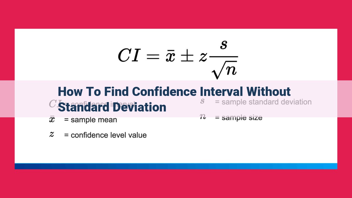
Now, let's dive into the formula:

Confidence Interval = Sample Mean ± Margin of Error

To calculate the margin of error, you'll use this formula:

Margin of Error = Critical Value * Standard Error

The standard error is a measure of how much your sample mean is likely to vary from the actual population mean. It's calculated as:

Standard Error = Population Standard Deviation / Square Root of Sample Size

In most cases, you won't know the population standard deviation. But fear not! You can use the sample standard deviation as an estimate:

Sample Standard Deviation / Square Root of Sample Size

Once you have your margin of error and critical value, you're ready to calculate your confidence interval.

Step-by-Step Example:

Let's say you're testing the effectiveness of a new fertilizer on corn yields. You collect a sample of 50 cornstalks and find that their average yield is 100 bushels per acre.

Let's assume you set a 95% confidence level (a common choice) and found that your critical value is 1.96.

Using the formula, we calculate the margin of error:

Margin of Error = 1.96 * 10 (estimated standard deviation) / √50

= 5.6

Now, we can plug everything into the confidence interval formula:

Confidence Interval = 100 ± 5.6

This means that we are 95% confident that the true average yield of corn in the population is between 94.4 and 105.6 bushels per acre.

By understanding confidence intervals, you can make informed decisions and draw reliable conclusions from your research or data analysis.

Related Topics: